Week 7 Update

Making the CNN work!

Goals from This Past Week

Team goal: Determine which algorithms/approaches we want to use in the end preprocessing and classification system.

Personal goals: Continue porting my classification code to OpenMV. Given additional training data from Tyler, I will test my classification algorithms for robustness.

Week 7 Milestone Goals

In our initial proposal, Tyler and I set the following goals for week 7. We did not revise these goals in our week 3 update

• Algorithm for combined segmentation and classification complete and ported over to H7

• LED matrix is built and controllable through the H7

Accomplishments

I spent this week working on the CNN. Tyler said he'd take the lead on porting my other classification algorithms to the H7, so I focused on creating a CNN for shape classification.

Getting the CNN Running on the H7

In prior weeks, the H7 would crash as soon as I tried to load the CNN without giving any error messages. Since the CNN is uploaded to the H7 as a single binary file and there were no error messages, it was very hard to know where to start debugging.

However, after some trial and error, I isolated the problem to be with the datatypes of the inputs and outputs of the network. I had them set to be unsigned integers instead of normal 8-bit integers. With a simple 2-line fix on the following lines, it could run without a problem!

converter.inference_input_type = tf.int8
converter.inference_output_type = tf.int8

Data Augmentation Attempt 1

After getting the CNN set up, I noticed that the network did not do very well with imperfect images. So, I set out to manually introduce noise into the training dataset.

I had already set up the network using a dataset on GitHub. This repository contains plenty of images that are all pre-labelled, so it was very easy to work with. I made 4 images out of each original image using the following transforms:

• Cropping by increasing or decreasing the area by a random number of pixels (between 0 and 5) on each side

• Adding salt and pepper noise to a random choice between the cropped/uncropped versions

Here are a few examples of the noisy versions of the images:

However, these updates caused the accuracy on images from Tyler to actually go down. My previous CNN got 10/12 shapes correct, but now it only got 8/12. The network seemed to default to classifying shapes as ovals, and it is impossible to see what within the CNN was causing this.

I realized that I would have to train the CNN on actual images from our system in order to get the accuracy higher in our system. That led me to my second attempt at creating a training dataset.

Data Augmentation Attempt 2

To use actual images from the H7 to train the CNN, I had to do a decent amount of work. Since OpenMV uses its own version of Python, I had to take Tyler's shape identification code and rewrite it so that it used functions available on Google Colab. Tyler provided colored 60x90 images of individual cards produced by his localization algorithm, and my code had to mimic the identification steps performed on each card. Below are some examples of card images from Tyler:

The steps to isolate the shapes are:

1. Remove the outer 5 pixels of the image to compensate for imperfections during the localization process

2. Erode the image to reduce noise

3. Zero out the white pixels leaving only pixels with color

4. Determine the number of shapes by using a mask to black out 1, 2, or 3 rectangles of size 52x26 (located where the shapes would be) and counting the remaining colored pixels. Increase the number of shapes that are blacked out until the number of remaining colored pixels falls below a pre-defined threshold. (see Tyler's blog post for more information about this)

5. Once the number of shapes is determined, extract the portions of a grayscale image of the card corresponding to each shape.

Steps 3 and 4 were the most involved. Tyler performed step 3 using a histogram function that is not available on Google Colab, so I approximated it by averaging the color RGB values across the image to determine the baseline white value. Once I calculate that threshold, I zero out all pixels identified as white. I also had to use a different threshold for each shape since the larger size of ovals made them leak more colored pixels into areas outside the pre-set rectangles that define where the shapes are. I know this wouldn't work in the real system (since it requires knowing the type of shape which is exactly what we are trying to figure out), but I figured it is okay since my algorithm is already very different from the one Tyler has for the final system. Step 4 also required a complete re-write, but the general algorithm remained the same.

Now, I was ready to begin adding noise. I generated 8 images from each original image, first by cropping the image in the same way I described earlier to create 3 new versions, and then rotating each of those 4 images (original and 3 cropped) 180 degrees. That gave training data that looks like the following:

I left out the salt and pepper noise here because it upset the coloration of the image in ways that would not appear in real life. See below for an example.

Below are 10 samples of my training data. In the end, I had 4000 total samples which I split between 3199 training images and 801 testing images (an 80-20 split).

CNN Architecture

I played around a lot with the CNN architecture to try to maximize accuracy without adding too many parameters. Here are some strategies I tested:

• Adding another convolution + pooling layer to decrease the number of nodes entering the dense layer

  • Although this adds more computations at runtime, it has the potential to decrease the memory requirement significantly through reducing the number of parameters

• Changing the number of channels in each convolution layer

• Adjusting the size of the convolution kernel (from 3x3 to 5x5)

• Increasing the area of max pooling to decrease the size of the data with consecutive layers

In the end, I settled on the following architecture:

Layer	Notes	Number of Parameters
2D Convolution	5x5 kernel, 6 channels	156
Max Pooling	2x2 window	0
2D Convolution	3x3 kernel, 6 channels	330
Max Pooling	2x2 window	0
Flatten	Converts image to flat array	0
Dense	Fully connected layer with 3 possible outputs (one for each type of shape)	1407

In total, this made a network of 1893 parameters. That is incredibly small for a CNN, which is perfect for applications on an embedded system. When the model is compiled into a single binary file that can run on the H7, it is only 5800 bytes (5.8% of the total SRAM available on the H7).

Results

After training for 50 epochs (which took about 3 minutes), this network achieved 100% accuracy on both the training and testing data! This may seem like overfitting, but the 801 testing datapoints were never seen during the training phase. It's ability to achieve 100% accuracy on completely unseen data makes me very confident that it will work well in implementation.

Since the CNN is now compiled into a single complete file, I can give Tyler that model file and Python file to apply it to an image.

Reflection on Week 7 Goals

Our goals for week 7, both in our original proposal and maintained in our week 3 update were as follows:

• Algorithm for combined segmentation and classification complete and ported over to H7

• LED matrix is built and controllable through the H7

I got the LED matrix working back in week 4, and the work Tyler and I did this week should finish up all the pieces for combined segmentation and classification on the H7. Tyler finished implementing a system to identify the number of shapes last week, and this week I built off that to classify the type of shape. The algorithms for color and fill are much simpler, and Tyler is finishing that up this week.

So, we do not require any modification to our week 7 goals, as we have successfully achieved them!

To summarize the major steps of our system, we start with an image that looks like this:

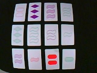
Then the H7 identifies the 12 cards and creates a cropped 60x90 image of each card. For example, here is the first row of the image above:

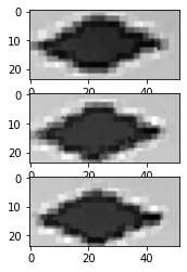
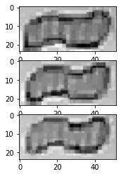
Then we run the classification algorithm on each card. This begins by identifying the colored pixels and testing various masks to determine how many shapes are on the card. Once we know the number of shapes, we isolate each one and run it through the CNN to classify the shape. The images of each shape are 26x52 grayscale images that look as follows:

Then, we run the color and fill algorithms that use the average ratios of the pixels' RGB values to classify the color and fill of the card. I described this process in my week 3 blog post.

Once each card has been classified, we run it through a set detection algorithm (described in my week 5 blog post). The sets are returned as tuples of 3 integers, where each integer represents the index of the card in the set.

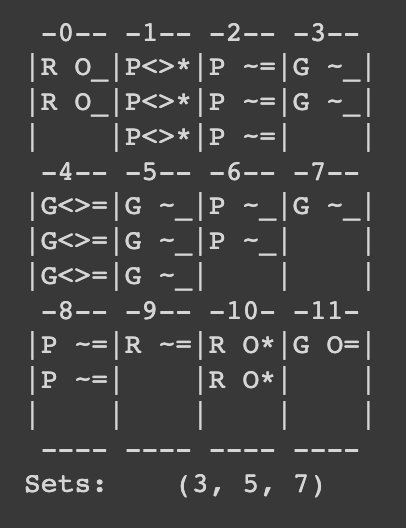
Lastly, these indices are used to light up the LED matrix. We have a matrix controller class that takes these indices and illuminates the corresponding set. The enclosure will make it clear which pixels correspond to each card, but for now I manually outlined each card's corresponding pixels in the image below:

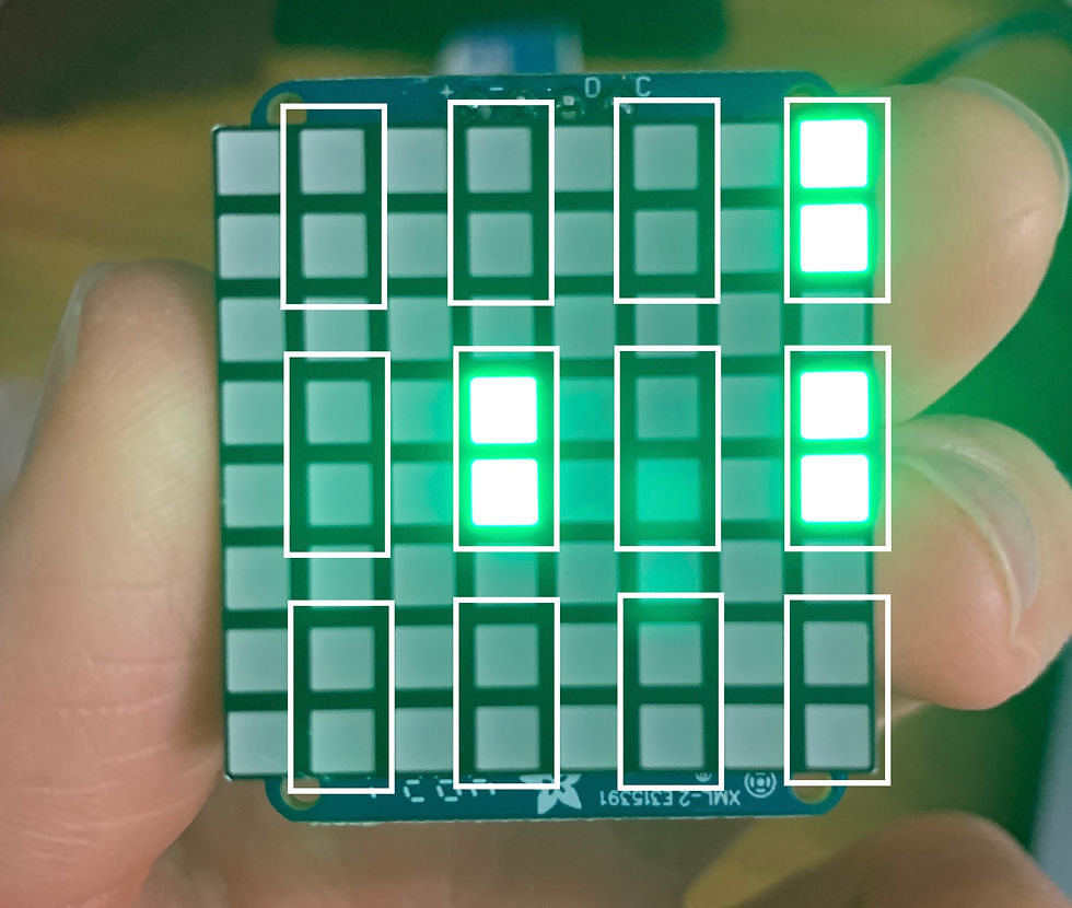
After comparing these pixels to the image above, I can verify that the illuminated pixels do indeed correspond to a valid set (empty green squiggles of with 1, 2, and 3 shapes)

So in summary, we were very successful in achieving our week 7 goals of being able to classify the cards on the H7! Now we can focus on testing and the physical design of the project.

Goals for Next Week

Team goals: Begin working on the physical design of the end product.

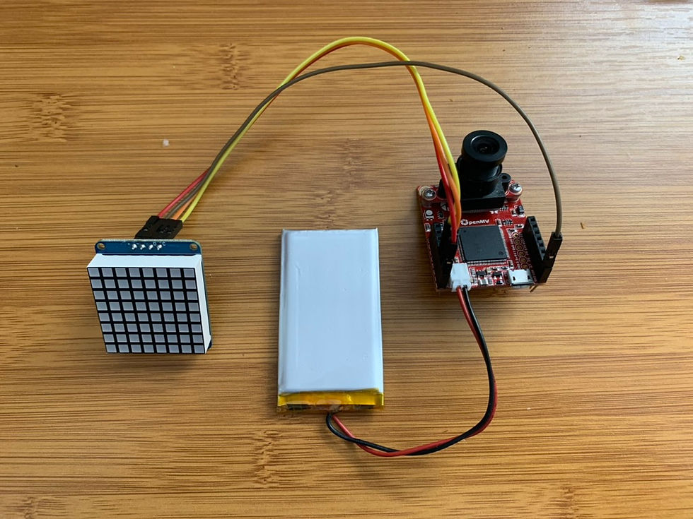
Personal goals: Find out how to run the H7 without being connected to a computer. This means finding a battery and making our program run by default (without requiring OpenMV).